Calibrated Probabilistic Forecasting of Household Power at the Edge

Grid operators increasingly manage congestion driven by rooftop solar, heat pumps and EV charging, yet most operational forecasts are still deterministic means. The decisions that matter live in the upper percentiles of feeder load, and reaching them takes calibrated, probabilistic models running close to the data. This note publishes a benchmark we built to test exactly that: quantile forecasting of both active (P) and reactive (Q) residential power, compressed until it runs on edge-class hardware, with every claim measured on a fully held-out test year.

The protocol

We used the public UCI Individual Household Electric Power Consumption dataset: four years (December 2006 to November 2010) of minute-resolution active and reactive power from a real residence, resampled to 15-minute means (138,352 intervals). The rules were strict: features use only past observations (lags, rolling statistics, calendar and solar-geometry terms); models train on 2007 to 2009 (about 104,000 intervals); evaluation happens only on the fully held-out year 2010 (about 28,000 intervals). The baseline is a seasonal-naive forecast with climatological residual quantiles fitted on training data alone. The metric is mean pinball loss across quantiles q = 0.1, 0.5 and 0.9.

Forecasts that track reality, with bands that mean what they say

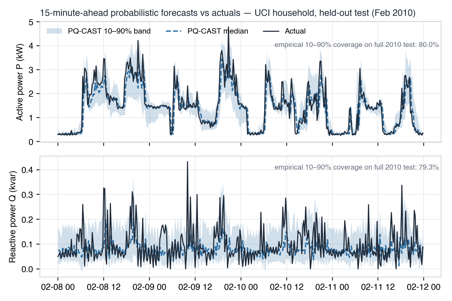
The property that decides whether an operator can act on a probabilistic forecast is calibration. Over the entire 2010 test year, the nominal 80% band empirically contains 80.0% of active-power observations and 79.3% of reactive-power observations. Bands like these are operational quantities, not decorative shading: a control room can set an alarm threshold on the upper quantile and know what the false-alarm budget actually is.

Skill and size

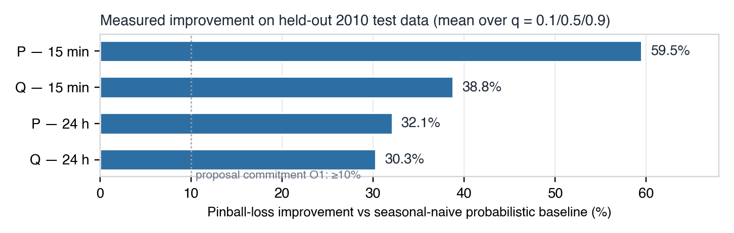
Quantile gradient boosting beat the baseline by 59.5% (P) and 38.8% (Q) at the 15-minute horizon, and by 32.1% and 30.3% at 24 hours. The serialised three-quantile model bundle measures 0.84 MB compressed, and a full three-quantile forecast computes in 0.52 ms on an ARM laptop-class CPU used as an edge proxy. In practical terms: this class of model runs comfortably on a Raspberry-Pi-class device sitting next to the meter, with training happening off-device and only inference plus light adaptation at the edge.

Honest caveats

This is one household, in one climate, against a deliberately simple baseline; a floor, not a ceiling. Beating a seasonal-naive forecast by 59% says little about beating a competent operational reference model, and a single French residence from 2006 to 2010 contains no rooftop PV, EV charging or heat-pump load. What the benchmark does establish, with numbers anyone can reproduce, is that calibrated probabilistic forecasting of both active and reactive power fits inside an edge budget with room to spare, and that the calibration machinery works on real, messy household data.

Why reactive power?

Residential reactive power is almost never forecast, yet voltage management at the grid edge depends on it. Q at a household is shaped by inverter control modes, motor loads and power-factor correction, which means it can be modelled conditionally on active power with physical structure. Treating Q as a first-class forecast target is, we think, one of the more useful and least crowded directions in grid-edge analytics.